The harmBounds package calculates stopping probabilities, defines stopping boundaries and generates plots for safety monitoring using an event based approach.
The idea is that under the null hypothesis of no safety concern, safety events are expected to occur at a frequency proportional to the randomization ratio. Assuming a single event per patient, we can do one sample binomial exact tests on the proportion of events in the treatment arm. In case of several events, we can use a beta-binomial framework, assuming a certain intra-class correlation coefficient. Evidence that the proportion of events in the treatment arm is higher than what is expected from randomization indicates a safety problem.
The safety monitoring can be done continuously after every event or at a pre-specified total number of events. The nominal test-wise alpha would be calibrated to obtain desired properties, such as a certain proportion of stopping under alternative scenarios of some degree of safety problems (the power). An overall type I error control can also be implemented but we would usually not recommend that for safety testing, as the consequence of a type II error (not stopping for safety if the treatment is not safe) is arguably worse than of a type I error (stopping if the treatment is safe).
The procedure is computationally efficient and fully reproducible, as all calculations are exact and derived in closed form from the binomial or the beta-binomial distribution.
Calculation of boundaries
Stopping boundaries can be calculated with function
getHarmBound. Let’s assume a trial with 10 safety interim
analyses after every 10 events (combined over both arms) up to a total
of 100 events and a nominal test-wise alpha of 0.025.
hb<-getHarmBound(nevents = seq(10, 100, by = 10), alpha_test = 0.025, pH0 = 0.5)
hb
#> $bounds
#>    events events_treatment events_control alpha_test
#> 1      10                9              1      0.025
#> 2      20               15              5      0.025
#> 3      30               21              9      0.025
#> 4      40               27             13      0.025
#> 5      50               33             17      0.025
#> 6      60               39             21      0.025
#> 7      70               44             26      0.025
#> 8      80               50             30      0.025
#> 9      90               55             35      0.025
#> 10    100               61             39      0.025
#>
#> $stopprob
#> $stopprob$`0.5`
#>    events  pH hyp   stop_prob cum_stop_prob
#> 1      10 0.5  H0 0.010742188    0.01074219
#> 2      20 0.5  H0 0.016405106    0.02714729
#> 3      30 0.5  H0 0.011266726    0.03841402
#> 4      40 0.5  H0 0.007307253    0.04572127
#> 5      50 0.5  H0 0.004798221    0.05051949
#> 6      60 0.5  H0 0.003217823    0.05373732
#> 7      70 0.5  H0 0.006730864    0.06046818
#> 8      80 0.5  H0 0.003002399    0.06347058
#> 9      90 0.5  H0 0.005713749    0.06918433
#> 10    100 0.5  H0 0.002449994    0.07163432
#>
#>
#> $opchar
#>     p cum_stop_prob expected_events hyp
#> 1 0.5    0.07163432        95.80595  H0
#>
#> attr(,"class")
#> [1] "harmbound" "list"
The data frame bounds specifies the boundaries at each interim analysis, events_treatment is the minimal number of events in the treatment arm that would lead to a stopping of the trial. The list stopprob contains stopping probability at each analysis for the null and optionally alternative hypotheses (see below). Data frame opchar shows the cumulative stopping probability and the expected number of events for each hypothesis.
In the example above, the overall type I error of the safety testing is 7.2%. The expected number of events (i.e. the average if the trial would be repeated) is 96. Typically, the trial might not be stopped at the last interim analysis, which can be specified using the maxevents option. The option only influences the expected events.
hb<-getHarmBound(nevents = seq(10, 100, by = 10), alpha_test = 0.025, pH0 = 0.5,
  maxevents = 150)
hb$opchar
#>     p cum_stop_prob expected_events hyp
#> 1 0.5    0.07163432        142.2242  H0
Alternative specification of rejection criteria
Instead of using an alpha for each test, we can also control the family-wise type I error rate at a specific level (even though we do not necessarily recommend that). Refer to the section on Choosing the test-wise alpha for more details.
hb<-getHarmBound(nevents = seq(10, 100, by = 10), alpha_total = 0.05, pH0 = 0.5,
  maxevents = 150)
hb$opchar
#>     p cum_stop_prob expected_events hyp
#> 1 0.5    0.05104241        144.7846  H0
The overall stopping probability under H0 (the type I error) is 5.1%, i.e. as close to 5% as possible (given the discrete nature of the test).If a strict control at 5% would required a alpha_total of 0.049 would have to be chosen.
Another more sensible option would be to target the type II error (or the power) for a specific alternative. This option requires the specification of an alternative, e.g. assuming that 60% of the events occuring in the experimental arm would indicate a safety problem (see the section on Operating characteristics for more details about the alternatives).
hb<-getHarmBound(nevents = seq(10, 100, by = 10), power = 0.8,
  pH0 = 0.5, pH1 = 0.6, maxevents = 150)
hb$opchar
#>     p cum_stop_prob expected_events hyp
#> 1 0.5     0.1980100       127.73727  H0
#> 2 0.6     0.8018467        62.47206  H1
Specifying alpha_total or power is much slower as
it relies on an iterative procedure ro determine the alpha used at each
step. It could make sense to first determine the alpha_test and
then use it directly in getHarmBound.
This can be done separately using function
getAlphaPerTest:
alphaPerTest<-getAlphaPerTest(nevents = seq(10, 100, by = 10),
  alpha_total = 0.05, pH0 = 0.5)

alphaPerTest
#> [1] 0.01760014

alphaPerTest<-getAlphaPerTest(nevents = seq(10, 100, by = 10),
  power = 0.8,  pH0 = 0.5, pH1 = 0.6)

alphaPerTest
#> [1] 0.07693005
Plotting of the boundaries
The boundaries can be plotted using harmboundPlot (or
the harmbound.plot-method):
hb<-getHarmBound(nevents = seq(10, 100, by = 10), alpha_test = 0.025, pH0 = 0.5,
  maxevents = 150)
plot(hb)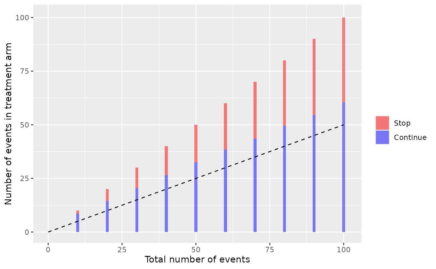
Where the bars indicate the time points of the interim analysis with the rejection region in red, and the dashed line represents the expectation (can be removed with ‘H0line = FALSE’)
Continuous monitoring could also be implemented:
hb<-getHarmBound(nevents = 0:100, alpha_test = 0.025, pH0 = 0.5,
  maxevents = 150)
plot(hb) 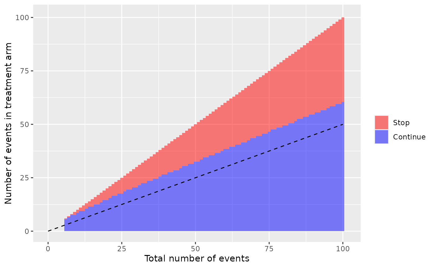
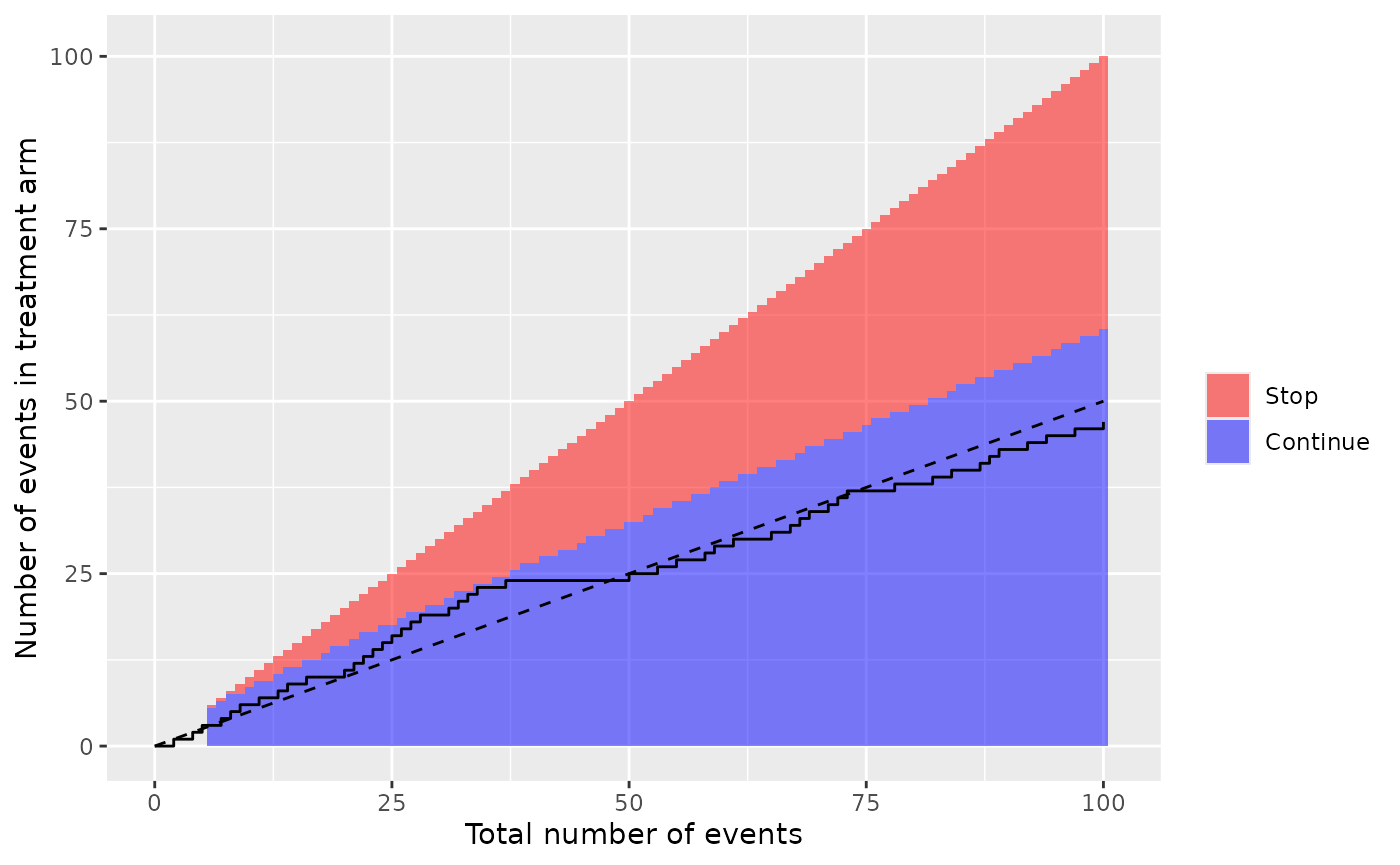
Observed data can be added as vector with 0 and 1, indicated the sequence of the arms in which events occurred (0 being the control and 1 the treatment arm). In this example, the boundary is not breached.
Operating characteristics
Stopping probabilities and expected number of events can be obtained
for alternative scenarios with the getHarmBound function.
The alternative hypothesis can be specified as
pH1: the proportion of the events in the treatment arm, with 0.5 being the null scenario for a 1:1 rando, and numbers from 0.5 to 1 indicating a safety problem.
rrH1: the risk ratio (treatment / control), with 1 being the null scenario and numbers >1 indicating a safety problem.
rdH1: the risk difference (treatment minus control), with 0 being the null scenario and numbers >0 indicating a safety problem. Here the control proportion (r0) has to be specified.
orH1: the odds ratio (treatment / control), with 1 being the null scenario and number >1 indicating a safety problem. Here the control proportion (r0) has to be specified.
To stay in the event-based setting, we recommend using the first two options (pH1 or rrH1).
#with proportion of events in the treatment arm:
hb<-getHarmBound(nevents = seq(10, 100, by = 10), alpha_test = 0.025, pH0 = 0.5,
  pH1 = 0.6, maxevents = 150)
hb
#> $bounds
#>    events events_treatment events_control alpha_test
#> 1      10                9              1      0.025
#> 2      20               15              5      0.025
#> 3      30               21              9      0.025
#> 4      40               27             13      0.025
#> 5      50               33             17      0.025
#> 6      60               39             21      0.025
#> 7      70               44             26      0.025
#> 8      80               50             30      0.025
#> 9      90               55             35      0.025
#> 10    100               61             39      0.025
#>
#> $stopprob
#> $stopprob$`0.5`
#>    events  pH hyp   stop_prob cum_stop_prob
#> 1      10 0.5  H0 0.010742188    0.01074219
#> 2      20 0.5  H0 0.016405106    0.02714729
#> 3      30 0.5  H0 0.011266726    0.03841402
#> 4      40 0.5  H0 0.007307253    0.04572127
#> 5      50 0.5  H0 0.004798221    0.05051949
#> 6      60 0.5  H0 0.003217823    0.05373732
#> 7      70 0.5  H0 0.006730864    0.06046818
#> 8      80 0.5  H0 0.003002399    0.06347058
#> 9      90 0.5  H0 0.005713749    0.06918433
#> 10    100 0.5  H0 0.002449994    0.07163432
#>
#> $stopprob$`0.6`
#>    events  pH hyp  stop_prob cum_stop_prob
#> 1      10 0.6  H1 0.04635740     0.0463574
#> 2      20 0.6  H1 0.09503665     0.1413940
#> 3      30 0.6  H1 0.08037764     0.2217717
#> 4      40 0.6  H1 0.06377080     0.2855425
#> 5      50 0.6  H1 0.05117939     0.3367219
#> 6      60 0.6  H1 0.04194665     0.3786685
#> 7      70 0.6  H1 0.07679694     0.4554655
#> 8      80 0.6  H1 0.03922701     0.4946925
#> 9      90 0.6  H1 0.06524712     0.5599396
#> 10    100 0.6  H1 0.03194760     0.5918872
#>
#>
#> $opchar
#>     p cum_stop_prob expected_events hyp
#> 1 0.5    0.07163432        142.2242  H0
#> 2 0.6    0.59188721         91.2001  H1
#>
#> attr(,"class")
#> [1] "harmbound" "list"
Note that stopprob is now of length two with a data frame for each condition.
We would stop in 7.2% of the trials under the null (no safety problem) and in 59.2% under the alternative (safety problem with 60% of the events in the treatment arm). Because of the higher probability of early stopping, the expected number of events is reduced from 142 under H0 to 91 under H1.
The (cumulative) stopping probabilities at each step can be plotted using absstopPlot or cumstopPlot (or the harmbound.plot-methods). We now using more than one alternative to make it more interesting:
hb<-getHarmBound(nevents = seq(10, 100, by = 10), alpha_test = 0.025,
  pH0 = 0.5, pH1 = c(0.6, 0.7, 0.8) , maxevents = 150)
plot(hb, which = "abs_stopping")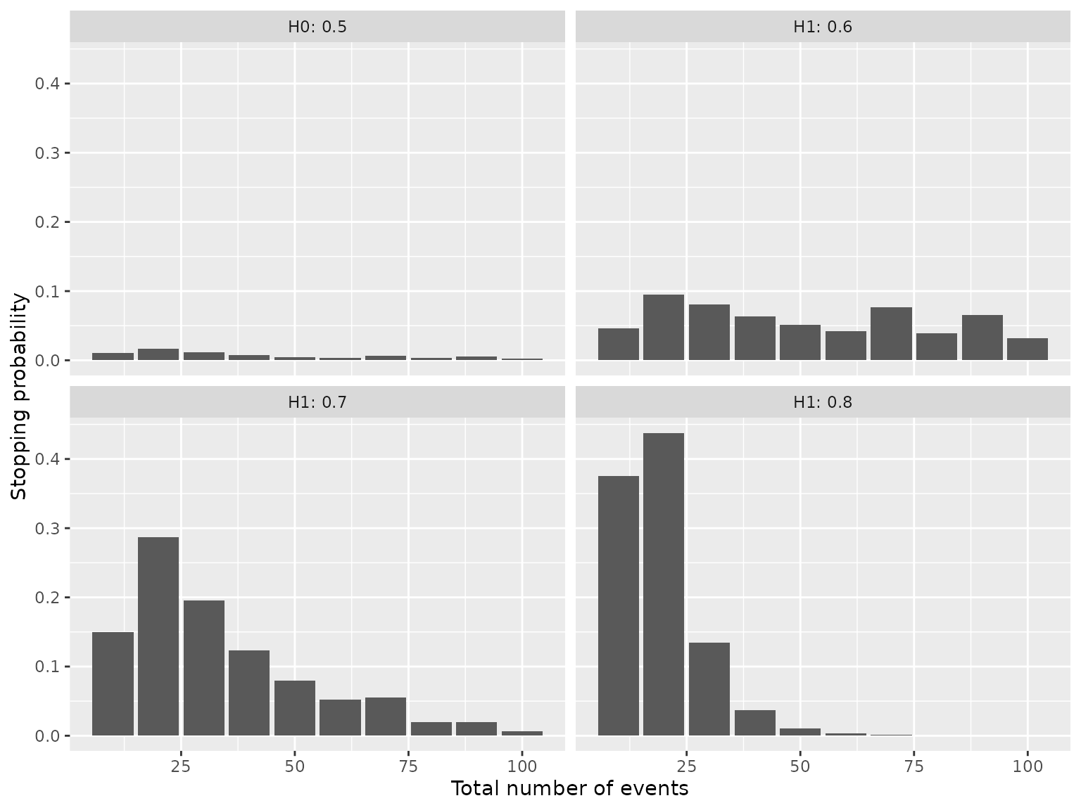
plot(hb, which = "cum_stopping")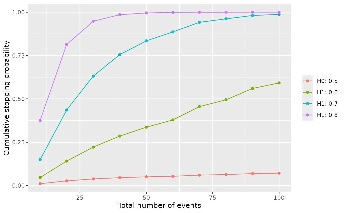
We can also specify a vector of alternatives and plot the cumulative stopping probabilities or the expected number of events for each alternative.
hb<-getHarmBound(nevents = seq(10, 100, by = 10), alpha_test = 0.025, pH0 = 0.5,
  pH1 = seq(0,1,l=100), maxevents = 150)
plot(hb, which = "opchar_stop")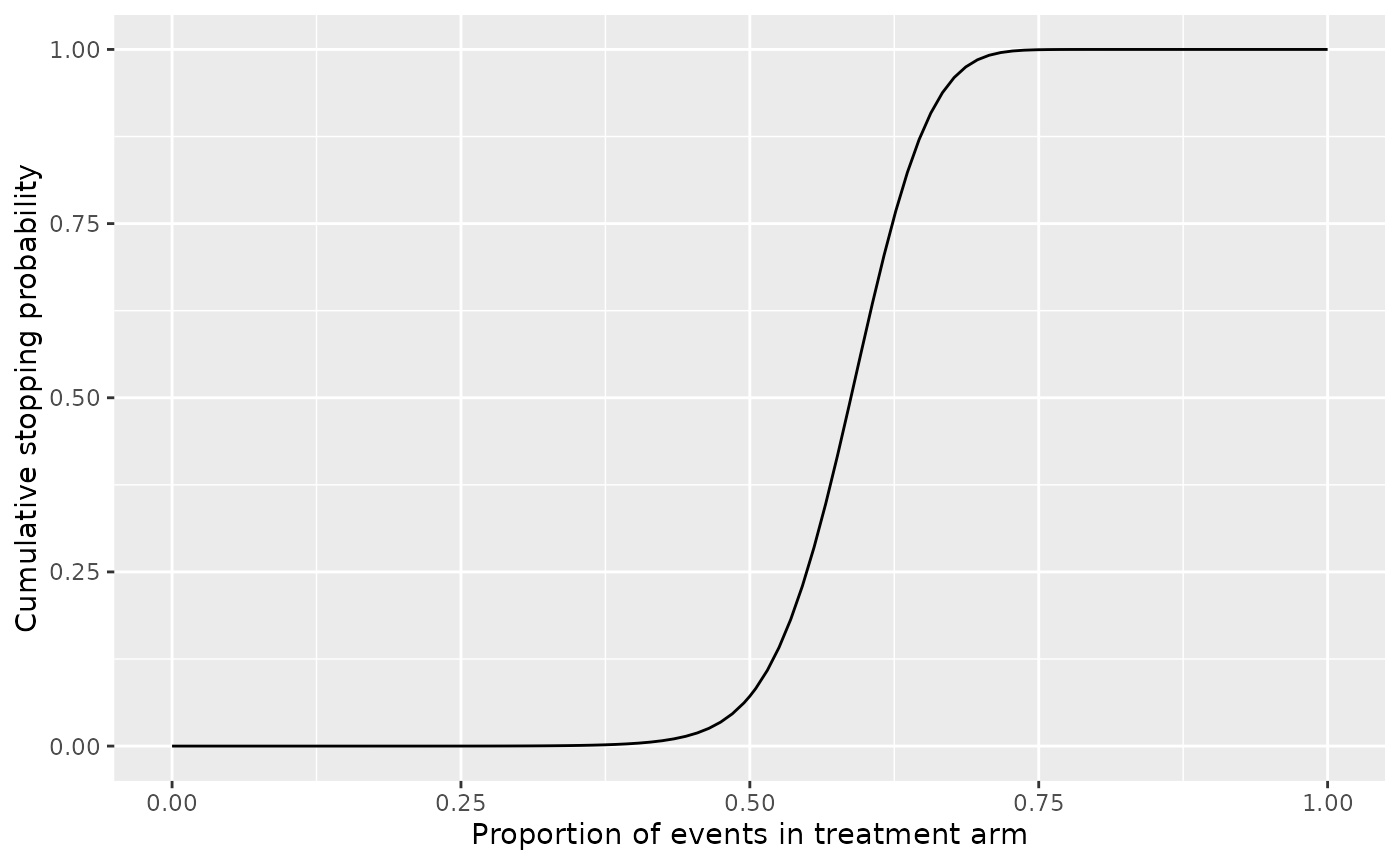
plot(hb, which = "opchar_n")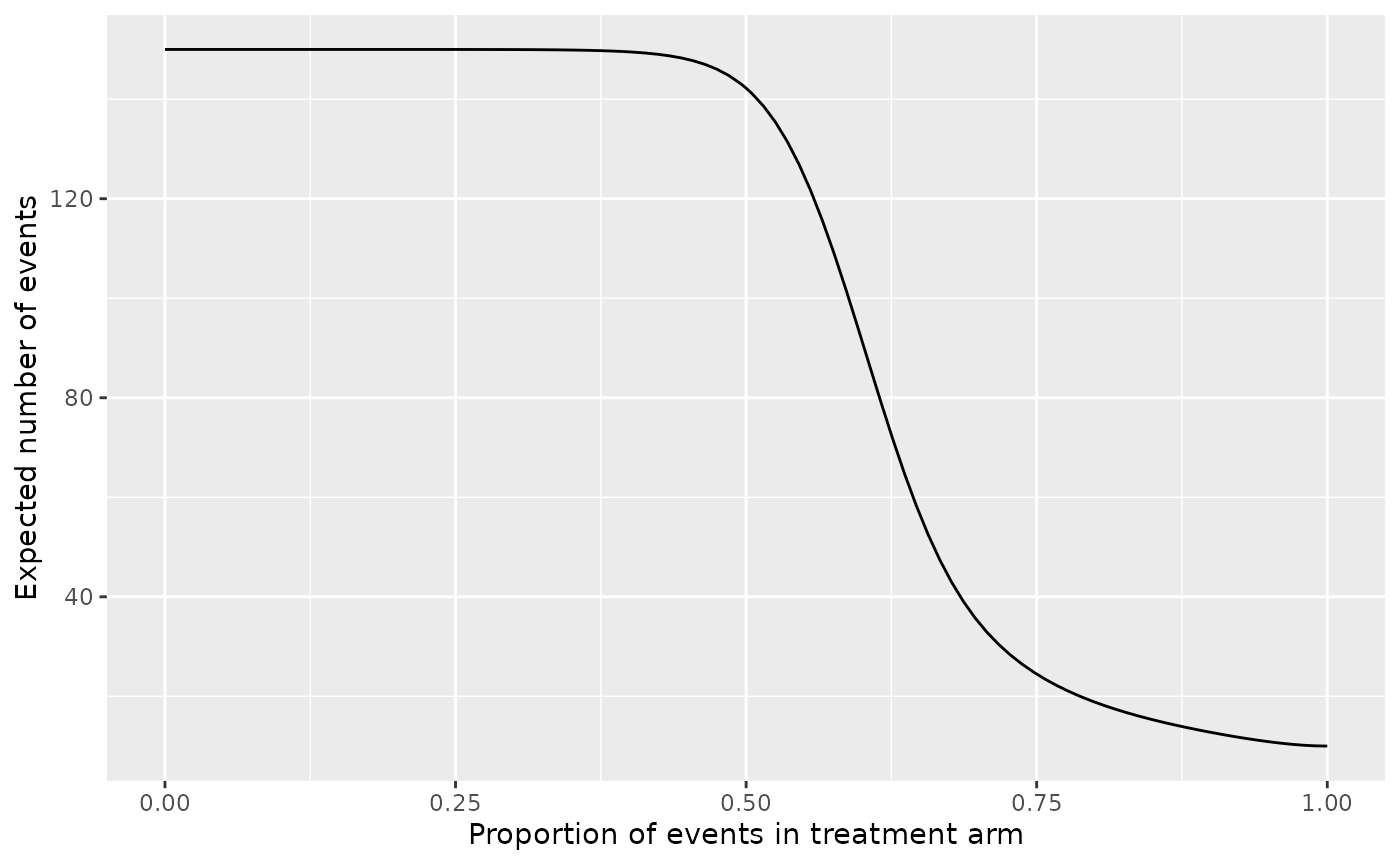
Choosing the test-wise alpha
To choose the test-wise alpha, we recommend to control the power rather than the type I error. I.e. to check that a sufficient proportion of trials are stopped under an appropriate alternative hypothesis (reflecting a safety problem).
A target power can be specified directly in getHarmbound
(see above).
To get a more complete picture, we would check the stopping probabilities for a grid of alphas:
alphaPerTest <- getAlphaPerTest(nevents = seq(10, 100, by = 10), pH0 = 0.5,
  alpha_total = 0.05)
alist<-c(0.001,0.01,alphaPerTest,0.025,0.05)

hbl<-lapply(alist,function(x)
  getHarmBound(nevents = seq(10, 100, by = 10), alpha_test = x,
  pH0 = 0.5, pH1 = seq(0,1,l=100), maxevents = 150)$opchar)

hbd<-data.frame(do.call(rbind,hbl),alpha=rep(alist,each=nrow(hbl[[1]])))
hbd$alpha<-as.factor(round(hbd$alpha,4))

ggplot(hbd, aes(x = p, y = cum_stop_prob, colour=alpha)) +
    geom_line() +
    ylab("Stopping probability") +
    xlab("Proportion of events in treatment arm") +
    scale_x_continuous(breaks=seq(0,1,by=0.1),limits=c(0.2,0.8)) +
    scale_y_continuous(breaks=seq(0,1,by=0.2))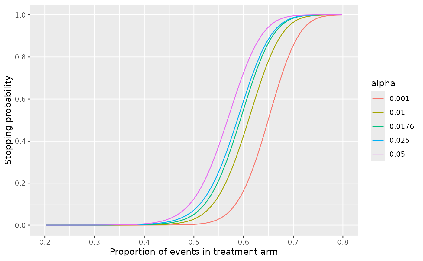
ggplot(hbd, aes(x = p, y = expected_events, colour=alpha)) +
    geom_line() +
    ylab("Expected number of events") +
    xlab("Proportion of events in treatment arm") +
    scale_x_continuous(breaks=seq(0,1,by=0.1),limits=c(0.2,0.8)) +
    scale_y_continuous(limits=c(0, 150))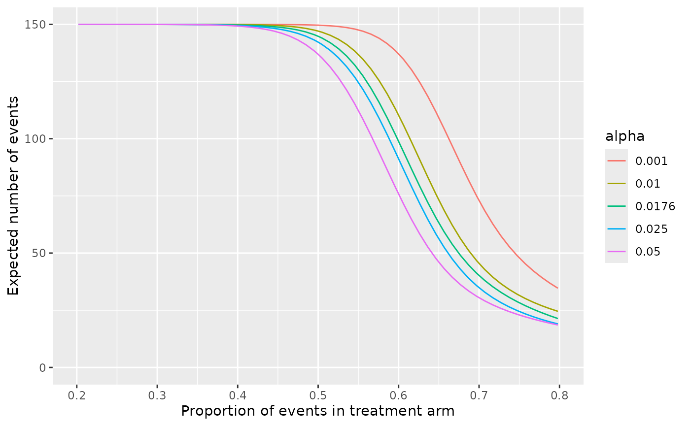
or on the transformed risk ratio scale:
alphaPerTest <- getAlphaPerTest(nevents = seq(10, 100, by = 10), pH0 = 0.5,
  alpha_total = 0.05)
alist<-c(0.001,0.01,alphaPerTest,0.025,0.05)

hbl<-lapply(alist,function(x)
  getHarmBound(nevents = seq(10, 100, by = 10), alpha_test = x, pH0 = 0.5,
  rrH1 = seq(0,10,l=100), maxevents = 150)$opchar)

hbd<-data.frame(do.call(rbind,hbl),alpha=rep(alist,each=nrow(hbl[[1]])))
hbd$alpha<-as.factor(round(hbd$alpha,4))
hbd$lrr<-log(hbd$rr)

ggplot(hbd, aes(x = rr, y = cum_stop_prob, colour=alpha)) +
    geom_line() +
    ylab("Stopping probability") +
    xlab("Risk ratio (treatment/control)") +
    scale_x_continuous(trans='log', breaks=c(0.5,0.75,1,1.5,2,3,4),
      minor_breaks=NULL,limits=c(0.5,5)) +
    scale_y_continuous(breaks=seq(0,1,by=0.2))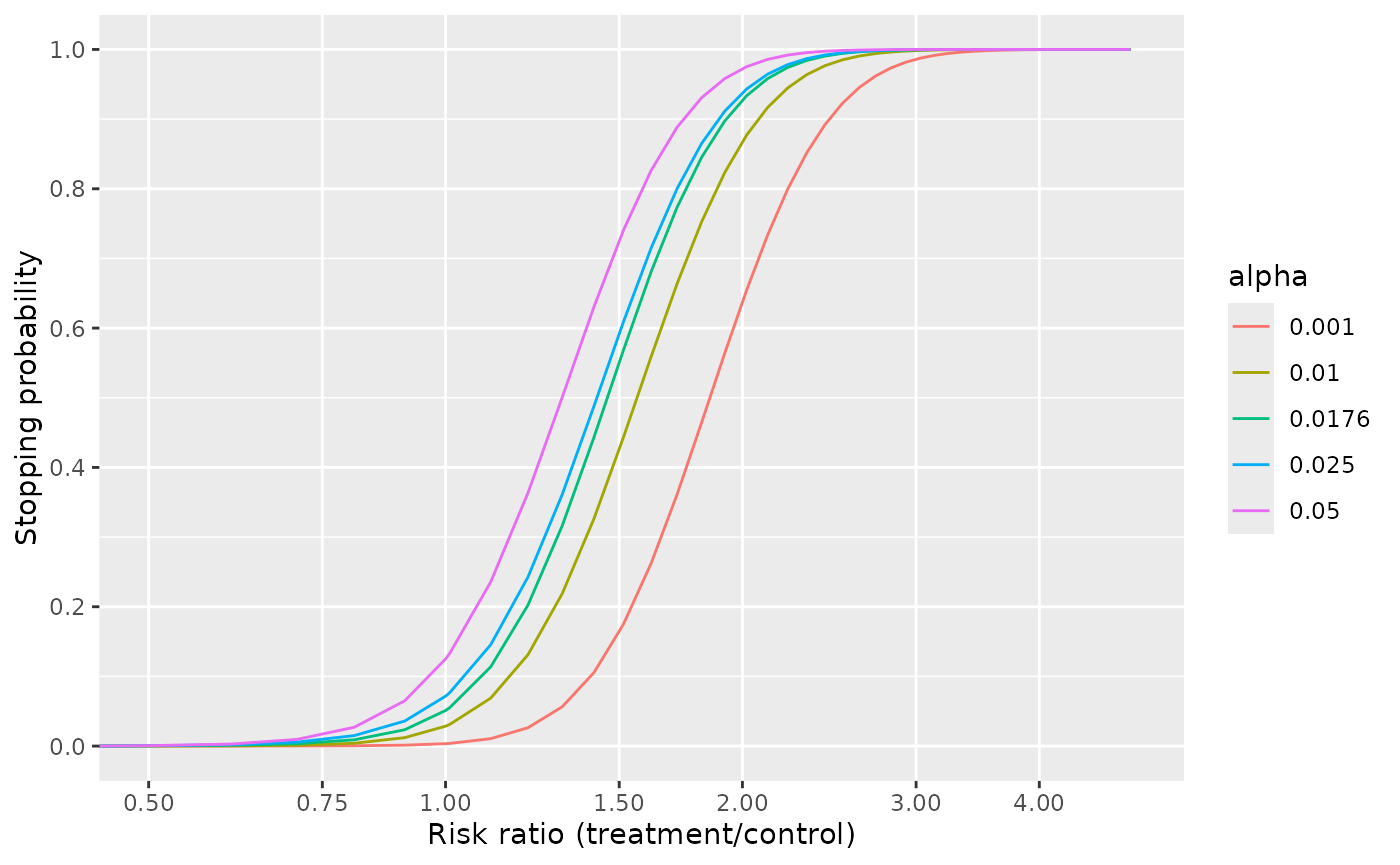
The test-wise alpha that leads to a reasonable stopping probability under an appropriate alternative can be selected. However, the steepness of the curve is not influenced by the alpha. We can only choose between making more type I or II errors but not reduce the overall error rate.
We could e.g. specify that at least 70% of the trials should be stopped if the risk of having a safety event increase by half (i.e. a risk ratio of 1.5), i.e. a test-wise alpha of close to 0.05. However, this would also lead to a stopping of 12.5% of the trials under the null.
On the other hand, if we control the type I error at 5% using a test-wise alpha of 0.0176, only 55% of the trials are stopped if there is a safety problem with a risk ratio of 1.5.
Further paramaters
The number of interim analyses has some impact on steepness and location of the curve, but it is rather limited, as long as the last interim analysis is at the same time point.
nelist<-list(c(100),c(50,100),c(10,20,50,100),
             seq(10, 100, by = 10),seq(10, 100, by = 1))

hbl<-lapply(nelist,function(x)
  getHarmBound(nevents = x, alpha_test = 0.025, pH0 = 0.5,
    pH1 = seq(0,1,l=100), maxevents = 150)$opchar)

nis<-unlist(lapply(nelist,length))
net<-unlist(lapply(nelist,function(x) paste(x,collapse = "/")))
net[[length(net)-1]]<-"every 10"
net[[length(net)]]<-"continous"
nism<-paste0(nis," (",net,")")
hbd<-data.frame(do.call(rbind,hbl),ni=rep(nism,each=nrow(hbl[[1]])))
hbd$ni<-factor(hbd$ni,levels=nism)

ggplot(hbd, aes(x = p, y = cum_stop_prob, colour=ni)) +
    geom_line() +
    ylab("Stopping probability") +
    xlab("Proportion of events in treatment arm") +
    scale_x_continuous(breaks=seq(0,1,by=0.1),limits=c(0.2,0.8)) +
    scale_y_continuous(breaks=seq(0,1,by=0.2)) +
    labs(colour="Number of IAs")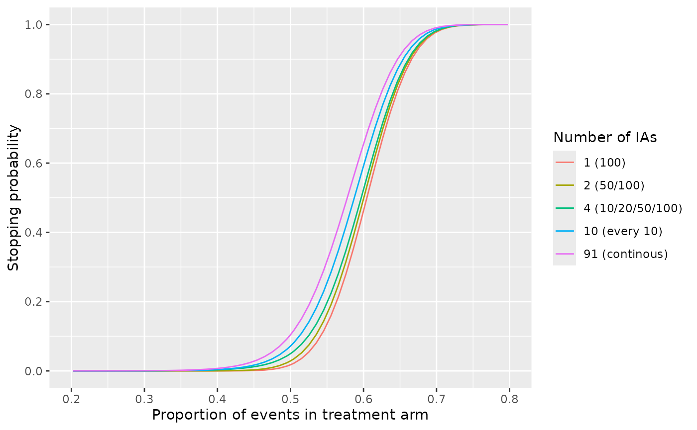
To substantially decrease the total error rates (i.e. get steeper curves), we would need a higher total number of events:
nelist<-list(seq(10, 20, by = 10),seq(10, 50, by = 10), seq(10, 100, by = 10),
  seq(10, 200, by = 10))

hbl<-lapply(nelist,function(x)
  getHarmBound(nevents = x, alpha_test = 0.025, pH0 = 0.5,
  pH1 = seq(0,1,l=100))$opchar)

nis<-unlist(lapply(nelist,max))
hbd<-data.frame(do.call(rbind,hbl),ni=rep(nis,each=nrow(hbl[[1]])))
hbd$ni<-as.factor(hbd$ni)

ggplot(hbd, aes(x = p, y = cum_stop_prob, colour=ni)) +
    geom_line() +
    ylab("Stopping probability") +
     xlab("Proportion of events in treatment arm") +
    scale_x_continuous(breaks=seq(0,1,by=0.1),limits=c(0.2,0.8)) +
    scale_y_continuous(breaks=seq(0,1,by=0.2)) +
    labs(colour="Total number of events")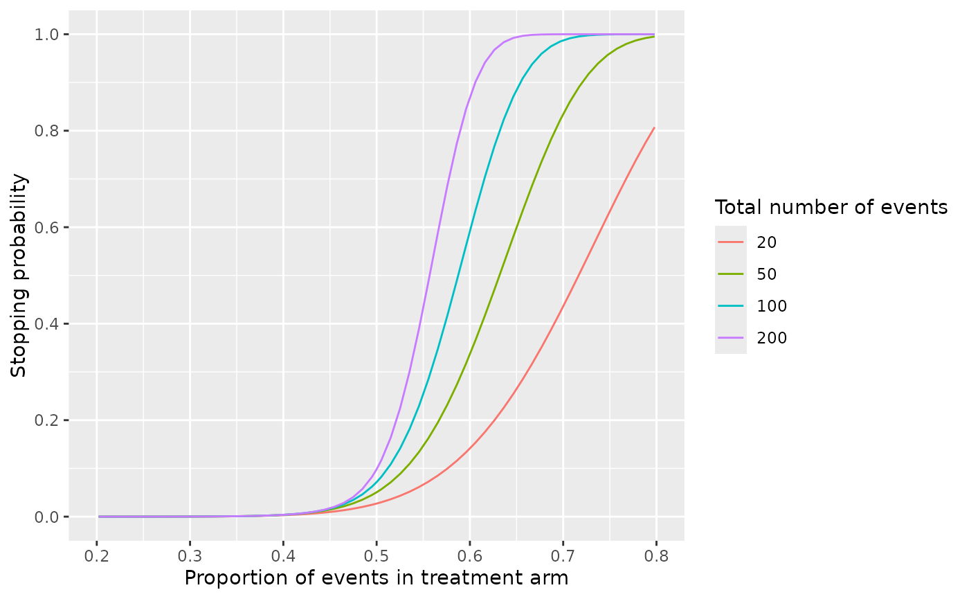
Correlated data
If patients can have more than one event, the binomial boundaries are no longer valid because the actual variance is increased. However, we can use a beta-binomial framework. That needs the specification of a intraclass correlation coefficient (icc).
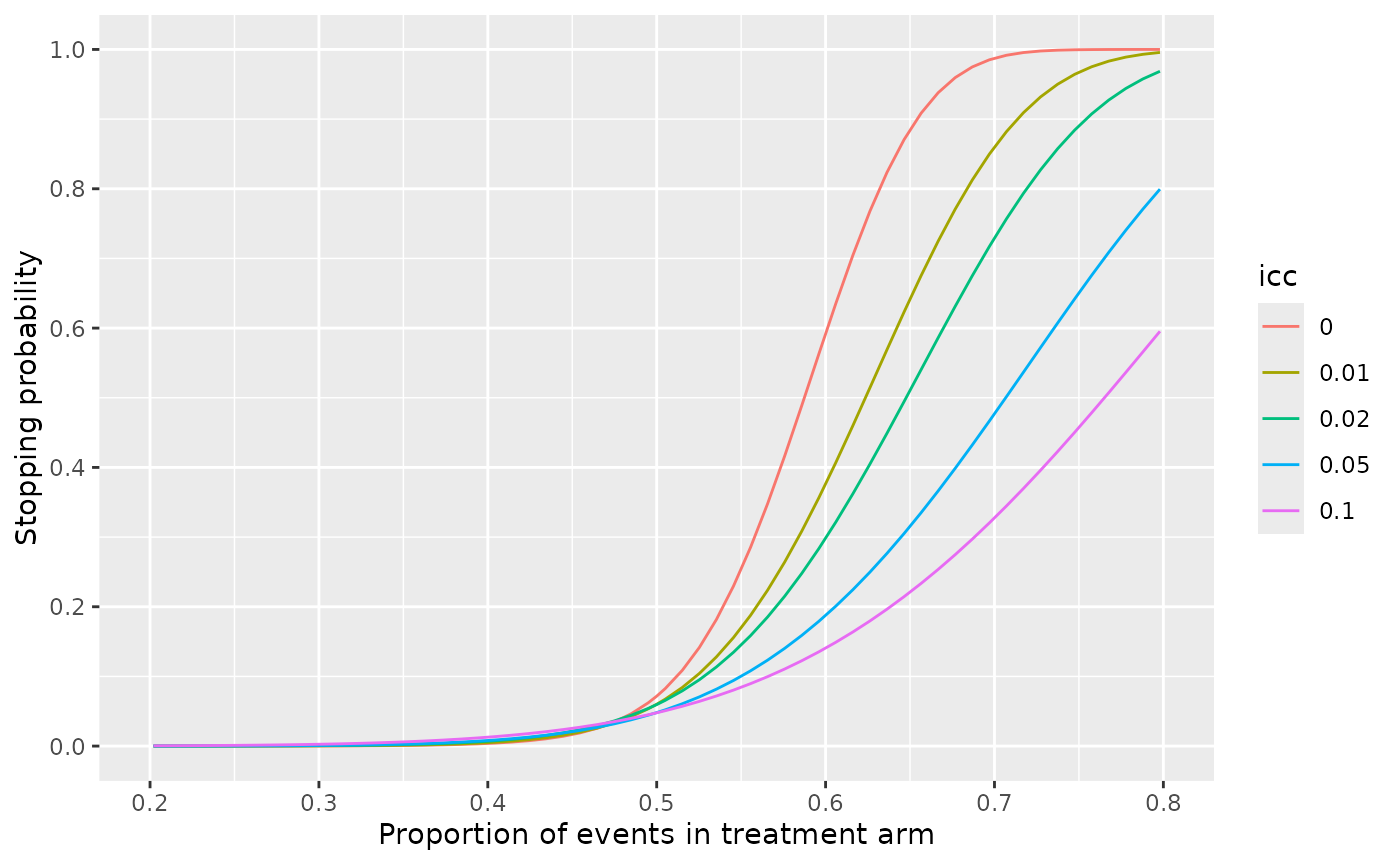
The overdispersion factor (or design effect) by which the beta-binomial variance exceeds the regular binomial variance corresponds to 1 + (n - 1) * icc and is printed by the function. Note that the effective sample size is reduced by that factor which results in a substantial loss of power, even for small ICCs.
For example, with an ICC of 0.05, we would only stop 19% of the trials with 60% events in the treatment arm, compared to 59% without correlation.
hb<-getHarmBound(nevents = seq(10, 100, by = 10), alpha_test = 0.025,
  pH0 = 0.5, pH1 = 0.6, maxevents = 150)
hb$opchar
#>     p cum_stop_prob expected_events hyp
#> 1 0.5    0.07163432        142.2242  H0
#> 2 0.6    0.59188721         91.2001  H1

hb<-getHarmBound(nevents = seq(10, 100, by = 10), alpha_test = 0.025,
  pH0 = 0.5, pH1 = 0.6, maxevents = 150, icc = 0.05)
#> [1] "Overdispersion factor: 1.45, 1.95, 2.45, 2.95, 3.45, 3.95, 4.45, 4.95, 5.45, 5.95"
hb$opchar
#>     p cum_stop_prob expected_events hyp
#> 1 0.5    0.04807753        144.5795  H0
#> 2 0.6    0.18755067        128.8848  H1
The effective sample size can be calculated using the overdispersion factor, which captures the increase in variance due to the correlation (the design effect). With an ICC of 0.05, the effective sample size is much smaller than the number of events:
nevents<-seq(10, 100, by = 10)
#overdispersion
ods<-1 + (nevents - 1) * 0.05
ods
#>  [1] 1.45 1.95 2.45 2.95 3.45 3.95 4.45 4.95 5.45 5.95
#effective sample size:
round(nevents/ods)
#>  [1]  7 10 12 14 14 15 16 16 17 17
We can plot this loss of power for different ICCs:
iccs<-c(0,0.01,0.02,0.05,0.1)

hbl<-lapply(iccs,function(x)
  getHarmBound(nevents = seq(10, 100, by = 10), alpha_test = 0.025,
  pH0 = 0.5, pH1 = seq(0,1,l=100), maxevents = 150, icc = x)$opchar)

hbd<-data.frame(do.call(rbind,hbl),icc=rep(iccs,each=nrow(hbl[[1]])))
hbd$icc<-as.factor(round(hbd$icc,2))

ggplot(hbd, aes(x = p, y = cum_stop_prob, colour=icc)) +
    geom_line() +
    ylab("Stopping probability") +
    xlab("Proportion of events in treatment arm") +
    scale_x_continuous(breaks=seq(0,1,by=0.1),limits=c(0.2,0.8)) +
    scale_y_continuous(breaks=seq(0,1,by=0.2))