Forest plots • forplot

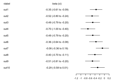
A package to generate forest plots.

Installation

forplot can be installed from github:


#install package using remotes
remotes::install_github("dcr-unibe-ch/forplot")

# load package
library(forplot)

Usage

forplot contains two main functions to build a forest plot.

genfobj requires a layout, specifying the elements to be plotted and a data frame (dat) with the data to be plotted and produces a list of class fobj.

The fobj can be modified using a set of helper functions or directly by changing the list.

plotfobj produces the plot from the fobj.

Example data

The package includes three data sets:

forplotdata: summary data with a 10 continuous variables
forplotdata_prop: summary data with 10 binary variables
forplotdata_bp: data with actual observation of forplotdata in a long format

data(forplotdata)
forplotdata
#>    vlabel  n1        n2  n3        n4            beta_format        beta
#> 1    out1 100 5.1 (0.9) 100 5.5 (1.0) -0.35 (-0.61 to -0.09) -0.35330456
#> 2    out2 100 5.0 (1.0) 100 5.6 (1.0) -0.52 (-0.80 to -0.24) -0.52192832
#> 3    out3 100 5.0 (1.2) 100 5.5 (1.0) -0.49 (-0.79 to -0.20) -0.49461488
#> 4    out4 100 4.8 (1.1) 100 5.5 (1.1) -0.70 (-1.00 to -0.40) -0.69983471
#> 5    out5 100 5.0 (1.1) 100 5.5 (1.1) -0.49 (-0.79 to -0.20) -0.49398774
#> 6    out6 100 5.0 (1.0) 100 5.3 (1.0) -0.36 (-0.64 to -0.08) -0.35838850
#> 7    out7 100 5.2 (1.1) 100 5.3 (0.9)  -0.08 (-0.36 to 0.19) -0.08429217
#> 8    out8 100 5.1 (1.0) 100 5.5 (1.1) -0.40 (-0.70 to -0.11) -0.40311974
#> 9    out9 100 4.9 (1.0) 100 5.4 (1.2) -0.51 (-0.81 to -0.20) -0.50709366
#> 10  out10 100 5.1 (1.1) 100 5.4 (1.1)  -0.29 (-0.58 to 0.01) -0.28700316
#>      beta_lci     beta_uci    p1
#> 1  -0.6122615 -0.094347655 0.008
#> 2  -0.8044964 -0.239360217 0.000
#> 3  -0.7938491 -0.195380711 0.001
#> 4  -1.0035691 -0.396100319 0.000
#> 5  -0.7928756 -0.195099871 0.001
#> 6  -0.6395674 -0.077209590 0.013
#> 7  -0.3567376  0.188153237 0.542
#> 8  -0.6955442 -0.110695309 0.007
#> 9  -0.8110643 -0.203123036 0.001
#> 10 -0.5822050  0.008198722 0.057

data(forplotdata_prop)
forplotdata_prop
#>    vlabel  n1       n2  n3       n4 prop1 prop2            beta_format  beta
#> 1    out1 100 48 (48%) 100 40 (40%)  0.48  0.40   8.0% (-6.7 to 22.7%)  0.08
#> 2    out2 100 38 (38%) 100 37 (37%)  0.38  0.37  1.0% (-13.4 to 15.4%)  0.01
#> 3    out3 100 47 (47%) 100 47 (47%)  0.47  0.47  0.0% (-13.8 to 13.8%)  0.00
#> 4    out4 100 54 (54%) 100 41 (41%)  0.54  0.41  13.0% (-1.7 to 27.7%)  0.13
#> 5    out5 100 45 (45%) 100 40 (40%)  0.45  0.40   5.0% (-9.7 to 19.7%)  0.05
#> 6    out6 100 51 (51%) 100 38 (38%)  0.51  0.38  13.0% (-1.7 to 27.7%)  0.13
#> 7    out7 100 47 (47%) 100 36 (36%)  0.47  0.36  11.0% (-3.6 to 25.6%)  0.11
#> 8    out8 100 44 (44%) 100 46 (46%)  0.44  0.46 -2.0% (-16.8 to 12.8%) -0.02
#> 9    out9 100 53 (53%) 100 33 (33%)  0.53  0.33   20.0% (5.6 to 34.4%)  0.20
#> 10  out10 100 54 (54%) 100 38 (38%)  0.54  0.38   16.0% (1.4 to 30.6%)  0.16
#>       beta_lci  beta_uci    p1
#> 1  -0.06714147 0.2271415 0.319
#> 2  -0.13418240 0.1541824 1.000
#> 3  -0.13834069 0.1383407 1.000
#> 4  -0.01723947 0.2772395 0.089
#> 5  -0.09684704 0.1968470 0.567
#> 6  -0.01656604 0.2765660 0.088
#> 7  -0.03571955 0.2557195 0.151
#> 8  -0.16786783 0.1278678 0.887
#> 9   0.05560305 0.3443969 0.007
#> 10  0.01364509 0.3063549 0.033

data(forplotdata_bp)
head(forplotdata_bp)
#>      value variable arm
#> 1 4.373546     var1   1
#> 2 5.183643     var1   1
#> 3 4.164371     var1   1
#> 4 6.595281     var1   1
#> 5 5.329508     var1   1
#> 6 4.179532     var1   1

forplotdata has a text column with the variable names (vlabel), text columns n[1-4] with the number of observations and descriptives for each arm (either mean (sd) or n(%)), the formatted treatment effect (beta_format) and the p-value (p1), and three numeric columns to draw the forest (beta, beta_lci and beta_uci).

In forplotdata_prop there are two further numeric columns with the proportion in each arm (prop1, prop2) to draw a srip plot.

forplotdata_bp has three columns with the actual observations of forplotdata with

value: the variable value (numerical),
variable: the variable name (factor), and
arm: the treatment arm (factor).

Generating the fobj with `genfobj`

genfobj requires the input of a layout and a data frame dat.

layout must be a character vector with elements t (text), f (forest), s[1-9] (strip), or b (boxplot).

For each t element, dat must contain a single column, for each f element three columns (point estimate, lower confidence limit, upper confidence limit, in that order), and for each s[1-9] the number of columns indicated in [].

The order of the columns must correspond to the layout.

A b element does not need a column in dat but the specifcation of obs, a data frame in a long format with columns value (the outcome value), variable (the outcome variable, safest as a factor to preserve the order in the plot), and arm (the treatment arm, safest as a factor to preserve the order in the plot)

We want to use forplotdata and generate a plot with a text columns with the label, the descriptives, the formatted effect and the p-value, and a forest for the beta.

fobj<-genfobj(dat = forplotdata, layout = c("t","t","t","t","t","t","f","t"))

The produced fobj is a list of length 5 with class fobj. It includes those elements:

dat and obs: the data
setup: the options from genfobj which has been given or assumed by default (i.e. layout, lheights, lwidths, y.at, ylim)
items: a list of length from layout with the options for each item
header: a list with the options for the header

class(fobj)
#> [1] "fobj" "list"
names(fobj)
#> [1] "dat"    "obs"    "setup"  "items"  "header"
fobj$setup
#> $layout
#> [1] "t" "t" "t" "t" "t" "t" "f" "t"
#> 
#> $lwidths
#> [1] 1 1 1 1 1 1 1 1
#> 
#> $lheights
#> [1] 0.1 1.0 0.1
#> 
#> $y.at
#>  [1] 10  9  8  7  6  5  4  3  2  1
#> 
#> $ylim
#> [1]  0.5 10.5
length(fobj$items)
#> [1] 8

By default, text items include these options:

names(fobj$item[[1]])
#> [1] "type"  "vname" "plot"  "text"

fobj$item[[1]]
#> $type
#> [1] "t"
#> 
#> $vname
#> [1] "vlabel"
#> 
#> $plot
#> $plot$x
#> [1] 0
#> 
#> $plot$type
#> [1] "n"
#> 
#> $plot$xlim
#> [1] 0 1
#> 
#> $plot$ylim
#> [1]  0.5 10.5
#> 
#> $plot$yaxt
#> [1] "n"
#> 
#> $plot$ylab
#> [1] ""
#> 
#> $plot$xlab
#> [1] ""
#> 
#> $plot$axes
#> [1] FALSE
#> 
#> $plot$xaxs
#> [1] "i"
#> 
#> $plot$yaxs
#> [1] "i"
#> 
#> 
#> $text
#> $text$x
#> [1] 0.5
#> 
#> $text$y
#>  [1] 10  9  8  7  6  5  4  3  2  1
#> 
#> $text$labels
#>  [1] "out1"  "out2"  "out3"  "out4"  "out5"  "out6"  "out7"  "out8"  "out9" 
#> [10] "out10"
#> 
#> $text$adj
#> [1] 0.5 0.5

type is the item type, vname is the variable in dat the item corresponds to, plot and text are the options used for plotting with base r.

The f items are more complex, including options for axis, points and arrows of the fores plots.

names(fobj$items[[which(fobj$setup$layout=="f")]])
#> [1] "type"   "vname"  "plot"   "axis"   "points" "arrows"

fobj$items[[which(fobj$setup$layout=="f")]]$type
#> [1] "f"

fobj$items[[which(fobj$setup$layout=="f")]]$vname
#> [1] "beta"

For the variable name, the first of the three variables used to specify the forest is used. Options for axis, point and arrows can be changed using helper functions (or directly in the list). Examples or shown below.

Plot the fobj

The fobj can be plotted using plotfobj

plotfobj(fobj)

And with a bit nicer widths, which can be given as options in genfobj or just be changing the fobj:

fobj$setup$lwidths <- c(0.3,0.4,0.6,0.4,0.6,1,1,0.5)

plotfobj(fobj)

Horizontal gridlines and stripes can be added with helper functions gridlines and stripes, which generate further elements in the fobj:

fobj<-gridlines(fobj)

fobj<-stripes(fobj)

names(fobj)
#> [1] "dat"       "obs"       "setup"     "items"     "header"    "gridlines"
#> [7] "stripes"

plotfobj(fobj)

Modify the items

All items, grid lines and stripes can be modified using helper functions or within the list directly.

For t items helper function t_options allows to use all options used in R graphics::text() function. That can be done for a specific t item by using the number or column name of the item, or for all (by keeping item=NULL):

fobj<-t_options(fobj = fobj, item = c("vlabel"), cex = 1.1, font = 2, col = "red", x=0.2, adj=0)

plotfobj(fobj)

For f items there are several helper function to modify the options for the different elements: f_axis, f_points, f_arrows. Also here, all options from graphics::axis(), graphics::points() and graphics::arrows() can be used. As we do only have one forest item, we do not have specify the item.

fobj<-f_axis(fobj = fobj, xlim = c(-1.1,0.2), at = c(-1,-0.6,-0.2,0.2), 
  tck = -0.03, mgp = c(2,0.5,0))

fobj<-f_points(fobj = fobj, pch = 16, cex = 1.5)

plotfobj(fobj)

With f_refline, a reference line can be added and with f_direction a label for the direction below the axis. Note that the footer height has to be increased to fit the direction label.

fobj<-f_refline(fobj, x = c(0, 0))

fobj<-f_direction(fobj, text = "A better    B better", line = 1.6)

fobj$setup$lheights[3]<-0.15

plotfobj(fobj)

To remove an added item, it can be set to NULL (or a new fobj could be generated):

fobj$items[[which(fobj$setup$layout=="f")]]$refline<-NULL

plotfobj(fobj)

Piping

The modifying elements can be piped. For example to reproduce the fobj from above:


genfobj(dat = forplotdata,
  layout = c("t","t","t","t","t","t","f","t"),
  lwidth = c(0.3,0.4,0.6,0.4,0.6,1,1,0.5),
  lheight = c(0.1,1,0.15)) |>
  gridlines() |>
  stripes() |>
  t_options(item = c("vlabel"), cex = 1.1, font = 2, col = "red", x=0.2, adj=0) |>
  f_axis(xlim=c(-1.1,0.2), at = c(-1,-0.6,-0.2,0.2), tck = -0.03, mgp = c(2,0.5,0)) |>
  f_points(pch = 16, cex = 1.5) |>
  f_refline(x = c(0, 0)) |>
  f_direction(text = "A better    B better", line = 1.6) |>
  plotfobj()

Arrowheads

When using xlim via f_axis, x-axis limits that are narrower then the confidence limits can be set (even though that is usually not recommended). The cap at the end of the confidence interval is then not plotted (as it is outside of the plotting region). However, directional arrowheads can help to make the distinction more prominent. Arrowheads can be modified via function f_arrows but it is not completely straightforward because arrows have to be drawn twice to have different heads on both sides (e.g. with code 1 and 2 and angles 30 and 90). The helper function f_cutarrows does that automatically:

# Modify data to generate some very wide limits:
dat<-forplotdata
dat$beta_lci[1]<-c(-3)
dat$beta_uci[2]<-c(3)
dat[3,c("beta_lci","beta_uci")]<-c(-3,3)
dat[4,c("beta","beta_lci")]<-c(-2,-3)
dat$beta_format<-paste0(sprintf("%2.2f",dat$beta),
  " (",sprintf("%2.2f",dat$beta_lci)," to ",
  sprintf("%2.2f",dat$beta_uci),")")

# Generate and plot fobj:
genfobj(layout = c("t","t","t","t","t","t","f","t"),
    dat = dat, lwidths = c(0.8,0.4,0.6,0.4,0.6,1,1,0.5)) |>
  f_axis(xlim=c(-1.5,1)) |>
  f_cutarrows() |>
  plotfobj()

The header

By default a header with the columns names is used and stored in the header element of fobj, which is a list of length 1 with these elements.

fobj$header
#> [[1]]
#> [[1]]$hlayout
#> [1] 1 2 3 4 5 6 7 8
#> 
#> [[1]]$text
#> [[1]]$text$x
#> NULL
#> 
#> [[1]]$text$y
#> [1] 0.5
#> 
#> [[1]]$text$labels
#> [1] "vlabel"      "n1"          "n2"          "n3"          "n4"         
#> [6] "beta_format" "beta"        "p1"         
#> 
#> [[1]]$text$adj
#> [1] 0.5 0.5

The header function can be used to modify the options using all options from graphics::text() As an extra element, the hlayout can be used to merge columns, i.e. to print a label over more than one column. And more than one header row can be specified using headernr, leading to a list of length > 1.

Let’s first just use different names, also including a line separator. Note that an empty character has to be included to leave column 1 and 8 empty. And the y is also modified to place the label it a bit higher.

fobj<-header(fobj = fobj,
  labels = c("","Arm A\nN","Arm A\nmean (sd)","Arm B\nN","Arm B\nmean (sd)",
    "Mean difference\n95% CI","","P-value"),
  y = 0.6)

plotfobj(fobj)

We could also merge the label for the effect over the format and forest columns. We would then change the layout to include one label twice. And remove the empty label for the forest column.

fobj<-header(fobj = fobj, hlayout = c(1,2,3,4,5,6,6,7),
  labels = c("","Arm A\nN","Arm A\nmean (sd)","Arm B\nN","Arm B\nmean (sd)",
    "Mean difference 95% CI","P-value"))

plotfobj(fobj)

In order to also merge to arm labels, we would need to header rows using option headernr, leading to a header list with length 2: As before we can use further graphics::text() options.

fobj<-header(fobj=fobj, hlayout = c(1,2,2,3,3,4,4,5),  headernr = 1,
    labels=c("","Arm A","Arm B","Mean diff (95% CI)","P-value"),
    y=0.9)

fobj<-header(fobj=fobj, hlayout = c(1,2,3,4,5,6,7,8), headernr = 2,
    labels=c("","N","Mean (sd)","N","Mean (sd)","","",""),y=0.3)


fobj$header 
#> [[1]]
#> [[1]]$hlayout
#> [1] 1 2 2 3 3 4 4 5
#> 
#> [[1]]$text
#> [[1]]$text$x
#> NULL
#> 
#> [[1]]$text$y
#> [1] 0.9
#> 
#> [[1]]$text$labels
#> [1] ""                   "Arm A"              "Arm B"             
#> [4] "Mean diff (95% CI)" "P-value"           
#> 
#> [[1]]$text$adj
#> [1] 0.5 0.5
#> 
#> 
#> 
#> [[2]]
#> [[2]]$hlayout
#> [1] 1 2 3 4 5 6 7 8
#> 
#> [[2]]$text
#> [[2]]$text$x
#> NULL
#> 
#> [[2]]$text$y
#> [1] 0.3
#> 
#> [[2]]$text$labels
#> [1] ""          "N"         "Mean (sd)" "N"         "Mean (sd)" ""         
#> [7] ""          ""         
#> 
#> [[2]]$text$adj
#> [1] 0.5 0.5


plotfobj(fobj)

Boxplots

For a more in-depth presentation of the data in each group, a boxplot can be added. However, it depends on the input of the actual observations as a data frame obs in a long format with the numerical outcome value (value), the variable name (variable, as a factor) and the treatment arm (arm, as a factor).

Note that the names of variable do not have to be the same as in the summary data (dat) but the order has to be kept (i.e. the first level of variable must correspond the first row in dat).

Boxplot layout can be controlled via helper functions b_boxplot and b_axis using all options available for graphics::boxplot() and graphics::axis().

fobj<-genfobj(dat = forplotdata, obs = forplotdata_bp,
  layout = c("t","t","t","t","t","b","t","f","t"),
  lwidths = c(0.6,0.4,0.6,0.4,0.6,1,1,1,0.5))

plotfobj(fobj)

Adding header gridlines and stripes:

fobj<-gridlines(fobj)

fobj<-stripes(fobj)

fobj<-header(fobj, hlayout = c(1,2,2,3,3,4,5,5,6),  headernr = 1,
    labels=c("","Arm A","Arm B","","Mean difference (95% CI)","P-value"),
    col = c(1,"red","blue",1,1),
    y=0.9)
fobj<-header(fobj, hlayout = c(1,2,3,4,5,6,7,8,9), headernr = 2,
    labels=c("","N","Mean (sd)","N","Mean (sd)","","","",""),
    col=1, y=0.3)

plotfobj(fobj)

Density plots

Density plots can be specified using layout item d and depend on the same data with the observations as the boxplots.

fobj<-genfobj(dat = forplotdata, obs = forplotdata_bp,
  layout = c("t","t","t","t","t","b","d","t","f","t"),
  lwidths = c(0.3,0.4,0.6,0.4,0.6,1,1,1,1,0.5))
 
fobj<-b_axis(fobj, xlim=c(0,9.5))

fobj<-gridlines(fobj)

fobj<-stripes(fobj)

fobj<-header(fobj, hlayout = c(1,2,2,3,3,4,5,6,6,7),  headernr = 1,
    labels=c("","Arm A","Arm B","","","Mean difference (95% CI)","P-value"),
    col = c(1,"red","blue",1,1,1),
    y=0.9)
fobj<-header(fobj, hlayout = c(1,2,3,4,5,6,7,8,9,10), headernr = 2,
    labels=c("","N","Mean (sd)","N","Mean (sd)","","","","",""),
    col=1, y=0.3)

plotfobj(fobj)

Options can be change via d_axis and d_lines using all options available for graphics::axis() and graphics::lines().

Note that the lines element of the d items is a nested list with variable and arm. Using d_lines, line options can be accessed all at once, over all variables for one arm, for all arms and one variable, or for a specific variable-arm combination via linenr. linenr is a vector of length two where the first element specifies the variable and the second the arm.

fobj<-genfobj(dat = forplotdata, obs = forplotdata_bp,
  layout = c("t","t","t","t","t","d","t","f","t"),
  lwidths = c(0.3,0.4,0.6,0.4,0.6,1,1,1,0.5))

#all lines:

fobj<-d_lines(fobj=fobj, lw=1.5)
plotfobj(fobj)

#only one arm:

fobj<-d_lines(fobj=fobj, linenr=c(NA,2), col=1)
plotfobj(fobj)

Different density curves could be added by using x and y options in d_lines (or the lines list in the fobj). Note that the y-position has to be shifted by y.at for each variable.

Strip plot for proportions

For binary outcomes and in particular for serious adverse event reporting a graphical representation of the proportion in both arms has been recommended.

A strip plot for the proportions can be added via s[1-9], where the number would indicate the number of points in the strip plot and the number of columns in the dat (usually two if there are two treatment arms). The “s” items then contains several points elements.

For example:

fobj<-genfobj(dat = forplotdata_prop,
  layout = c("t","t","t","t","t","s2","t","f","t"),
  lwidths = c(0.3,0.4,0.6,0.4,0.6,1.0,1.2,1,0.5))

plotfobj(fobj)

Options can be modified via s_axis, s_hline and s_points using all options available for using all options available for graphics::axis(), graphics::abline() and graphics::points().

Note that for points, each sub-item has can be specified separately using pointnr (e.g. to specify colors).

Left and right borders can be added via s_borders.

fobj<-s_axis(fobj=fobj, xlim = c(0,1), 
  at = seq(0,1,by=0.25), labels = seq(0,100,by=25))

fobj<-s_points(fobj=fobj, pch = 16, cex=1.5)

fobj<-s_points(fobj=fobj, pointnr = 1, col = "red")

fobj<-s_points(fobj=fobj, pointnr = 2, col = "blue")

fobj<-s_borders(fobj)

fobj<-gridlines(fobj)

plotfobj(fobj)

Combine plots

plotfobj also works with a list of fobj as long as the layout has the same length. If the lwdiths vary, the average is taken.

#define common lwidths
commonlwidths<-c(0.3,0.4,0.6,0.4,0.6,1,1,1,0.5)

#prepare first fobj
fobj1<-genfobj(dat = forplotdata, obs = forplotdata_bp,
  layout = c("t","t","t","t","t","b","t","f","t"),
  lwidths = commonlwidths)

fobj1$setup$lheights[1]<-0.2
fobj1$setup$lheights[3]<-0.2

fobj1<-gridlines(fobj = fobj1)
fobj1<-stripes(fobj = fobj1)

fobj1<-header(fobj = fobj1, hlayout = c(1), headernr = 1,
    labels=c("Continuous variables"),
    col = 1, y = 0.9, font = 2, cex=1.2)

fobj1<-header(fobj = fobj1, hlayout = c(1,2,2,3,3,4,5,5,6),  headernr = 2,
    labels=c("","Arm A","Arm B","","Mean difference (95% CI)","P-value"),
    col = c(1,"red","blue",1,1), y = 0.45, font = 1, cex = 1)

fobj1<-header(fobj = fobj1, hlayout = c(1,2,3,4,5,6,7,8,9), headernr = 3,
    labels=c("","N","Mean (sd)","N","Mean (sd)","","","",""),
    col = 1, y = 0.15, font = 1, cex = 1)


#prepare second fobj
fobj2<-genfobj(dat = forplotdata_prop,
  layout = c("t","t","t","t","t","s2","t","f","t"),
  lwidths = commonlwidths)

fobj2$setup$lheights[1]<-0.2
fobj2$setup$lheights[3]<-0.2

fobj2<-s_axis(fobj = fobj2, xlim = c(0,1), 
  at = seq(0,1,by=0.25), labels = seq(0,100,by=25))

fobj2<-s_borders(fobj = fobj2)

fobj2<-gridlines(fobj = fobj2)
fobj2<-stripes(fobj = fobj2)

fobj2<-header(fobj = fobj2, hlayout = c(1), headernr = 1,
    labels=c("Binary variables"),
    col = 1, y = 0.9, font = 2, cex=1.2)

fobj2<-header(fobj = fobj2, hlayout = c(1,2,2,3,3,4,5,5,6),  headernr = 2,
    labels=c("","Arm A","Arm B","Proportion (%)","Odds ratio (95% CI)","P-value"),
    col = c(1,"red","blue",1,1), y = 0.45, font = 1, cex = 1)

fobj2<-header(fobj = fobj2, hlayout = c(1,2,3,4,5,6,7,8,9), headernr = 3,
    labels=c("","N","n (%)","N","n (%)","","","",""),
    col = 1, y = 0.15, font = 1, cex = 1)


#plot list:
plotfobj(fobj = list(fobj1, fobj2))

Combining plots can also be used to get different scaling for the plots of the individual variables. Assume we would like to present a number of differently scaled continuous variables with boxplots and densities:

set.seed(1)

fobj<-vector(10,mode="list")

for (i in 1:10) {
  
  #modify the data
    obs<-forplotdata_bp[forplotdata_bp$variable==paste0("var",i),]
    obs$value<-obs$value + runif(1,-10,10)
    obs$variable<-factor(obs$variable)
    
    dat<-cbind(forplotdata[i,1:5],"")
    dat$n2<-paste0(sprintf("%1.1f",mean(obs$value[obs$arm==1]))," (",
    sprintf("%1.1f",sd(obs$value[obs$arm==1])),")")
    dat$n4<-paste0(sprintf("%1.1f",mean(obs$value[obs$arm==2]))," (",
    sprintf("%1.1f",sd(obs$value[obs$arm==1])),")")
    
    #generate individual fplots
    fobji<-genfobj(dat = dat, obs = obs,
        layout = c("t","t","t","t","t","b","t","d"), 
        lwidths = c(0.3,0.4,0.6,0.4,0.6,1,0.1,1),
        lheights = c(0.2,1,0.25))
    
    fobji<-b_axis(fobji, cex.axis=0.8, mgp=c(0,0.3,0), tck=-0.1)
    fobji<-d_axis(fobji, cex.axis=0.8, mgp=c(0,0.3,0), tck=-0.1)
    
    #header for first fplot only
    if (i!=1) { 
        fobji$header<-NULL
    } else {
        
        fobji<-header(fobj = fobji,
      hlayout = c(1,2,2,3,3,4,5,6), headernr = 1,
            labels=c("","Arm A","Arm B","Boxplot","","Density"),
            col = c(1,"red","blue",1,1), y = 0.9)

        fobji<-header(fobj = fobji,
      hlayout = c(1,2,3,4,5,6,7,8), headernr = 2,
            labels=c("","N","mean (sd)","N","mean (sd)","","",""),
            col = 1, y = 0.35)
        
        fobji<-gridlines(fobji,gridnr=2)
    }
    
    #collect
    fobj[[i]]<-fobji
    
}

#adapt top header and bottom footer
fobj[[1]]$setup$lheights[1]<-1
fobj[[length(fobj)]]$setup$lheights[3]<-0.5

#plot the list of fobj
plotfobj(fobj)

`forplot`

Installation

Usage

Example data

Generating the fobj with `genfobj`

Plot the fobj

Modify the items

Piping

Arrowheads

The header

Boxplots

Density plots

Strip plot for proportions

Combine plots

Links

License

Citation

Developers

forplot

Installation

Usage

Example data

Generating the fobj with genfobj

Plot the fobj

Modify the items

Piping

Arrowheads

The header

Boxplots

Density plots

Strip plot for proportions

Combine plots

Links

License

Citation

Developers

`forplot`

Generating the fobj with `genfobj`